Use keyboard arrow keys to
advance ( → ) and
go back ( ← )
Type “s” to see speaker notes
Type “?” to see other keyboard shortcuts
The Data Analysis Pipeline
a grammar for transforming data frames
library(dplyr) OR library(tidyverse)
dplyr (pronounced dee-ply-er, a play on words with “data” and “pliers”) is a useful R package we’ll discuss in this section. The various functions we’ll use, like select, filter, and mutate are all functions that belong to the dplyr package.
Just as a reminder, in R, we bring in the functionality of a package by using the library() command. Because dplyr forms part of the tidyverse suite of packages, we can bring in the useful functions of dplyr by either using the library(dplyr) command or the library(tidyverse) command.
The idea behind dplyr is that any data analytic task can be broken down into a small number of basic or atomic tasks, and there should be a consistent way to specify each atomic task - a grammar.
As we will see in this last section, each dplyr function takes a data frame, does something with it, and then returns a modified data frame as its output. Dplyr functions can be strung together to create powerful data analysis pipelines in just a few lines of code.
Subsetting Data
Often, you have a large data frame but want to create a graph or analyze data from only a small part of it. The dplyr package, part of the larger tidyverse set of packages, works great for this purpose.
Let’s look at how you can subset a data frame (choose only certain columns and/or rows) by using dplyr.
Subsetting Columns vs Rows
dplyr provides two functions for subsetting data frames: select() for subsetting columns, and filter() for subsetting rows:
select() reshapes data so that it includes only the columns you specify.
filter() reshapes data so that it includes only the rows that meet your conditions.
select()
select(data_frame, ...)
Let’s look at select() first. The select() function extracts columns from a data frame, using the column name(s) as argument(s).
select() takes a data frame as its first argument. After that it takes any number of additional arguments that specify the names of the columns that you want to pick.
We extract columns by name with code that looks like this, and we replace the three dots with the names of the columns we want to keep.
select()
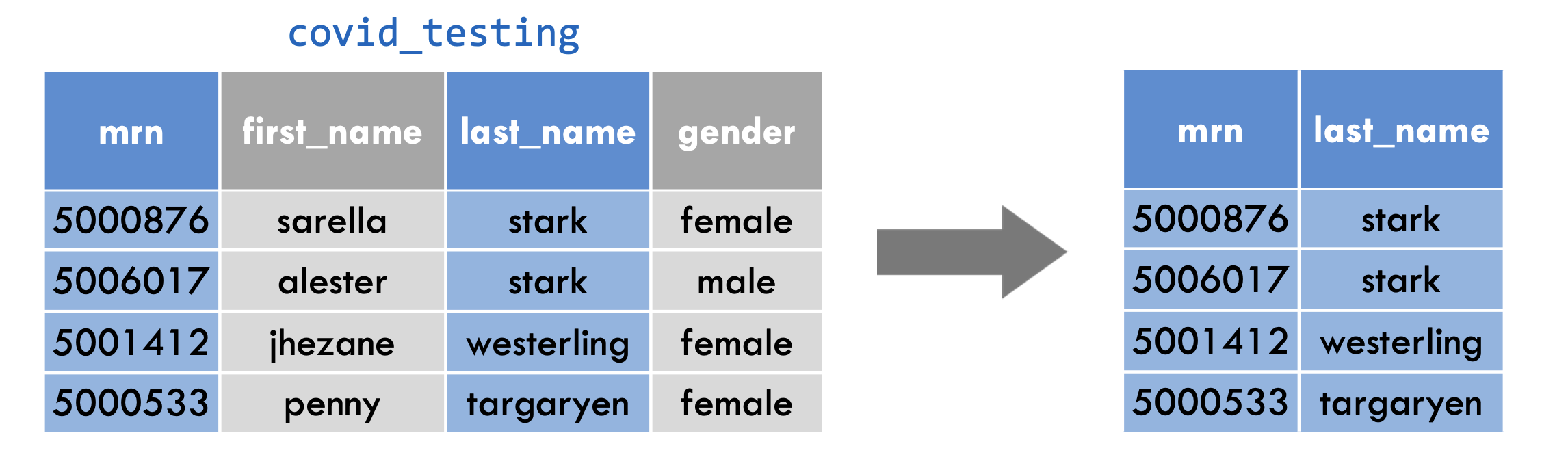
select(covid_testing, mrn, last_name)
Let’s examine the code on this slide.
This select statement will take the data frame covid_testing, and return a new data frame that only has the columns mrn and last_name, shown here in blue to help you visualize this transformation.
An important point to note here is that select will not modify the original data frame but simply returns the altered data frame you asked for, without saving it automatically.
If you write the select statement like this it will simply print out the result in the console or in your R Markdown document. If you want to capture the modified data frame you need to assign it to a named object.
Your Turn #1
Which of the following will select the first_name column from the covid_testing data frame and capture the result in a data frame named newdata?
A) newdata = select(first_name, covid_testing)
B) newdata <- select(covid_testing, first_name)
C) select(newdata, covid_testing, first_name)
D) newdata <- select(covid_testing, First_Name)
E) Both B and D
Type your response in the chat!
Great, we have some folks saying , others are suggesting . The answer is B.
A isn’t correct because the arguments are in the wrong order. The first argument in the tidyverse functions we’re studying today is always going to be the data frame you want to work with. That means the first argument should be covid_testing.
C isn’t correct because you have to use the assignment arrow to save the new, one-column-only data frame to an object called newdata. You don’t pass the name you want to apply to the object as an argument.
D isn’t right because capitalization matters! First name with a capital F is not the same as first name with a lower case f.
So E is also clearly incorrect.
filter()
filter(data_frame, ...)
One of the most important dplyr functions to know about is filter(). filter() extracts rows, and it does that based on logical criteria , or a condition that can be evaluated to be true (keep that row as part of our subset) or false (don’t keep that row).
Like select(), filter() takes a data frame as its first argument. The second argument is a condition or logical test. R then performs that logical test on each row of the dataset and returns all rows in which the logical test was true.
To extract rows that meet logical criteria, we write code that looks like this, and we replace the three dots with the condition we want to test for each row.
filter()
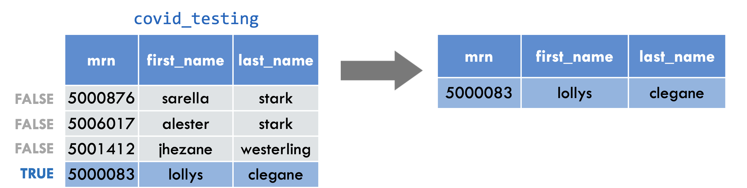
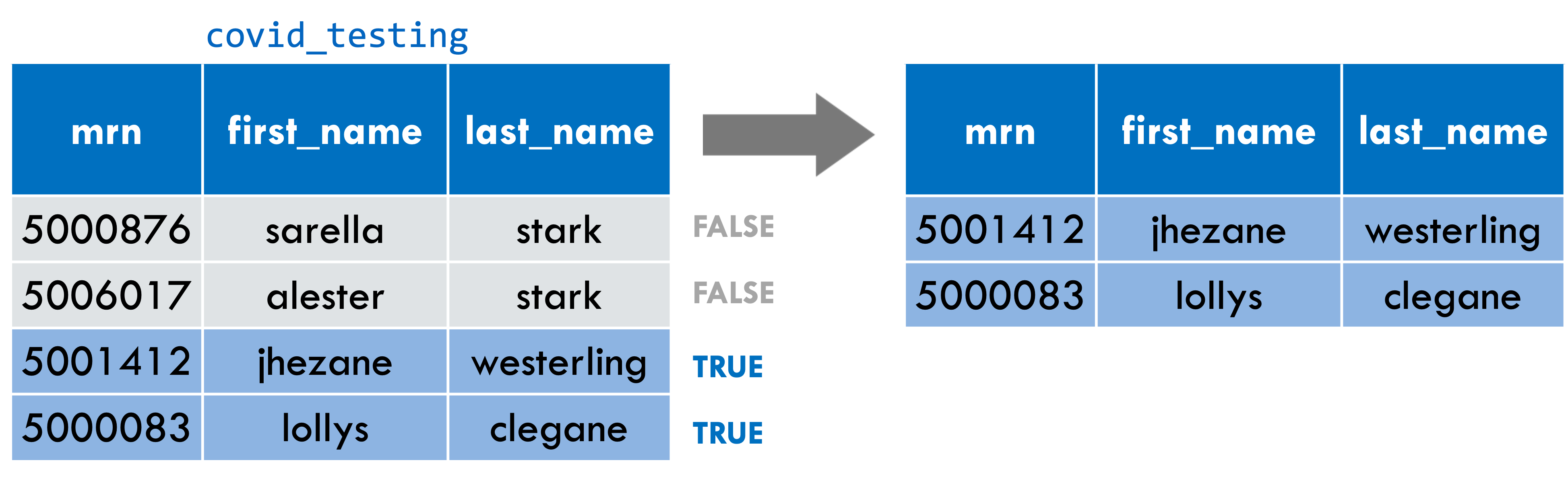
filter(covid_testing, mrn == 5000083)
To give you an example: the logical test here is whether or not the mrn value is equal to 5 00 00 83. This is false for the first three rows. In these rows, the mrn value is something else. For the 4th row, however, it is true that the mrn value is equal to 5 00 00 83.
This filter statement will return a data frame that only contains the 4th row, in which the logical condition is true , as shown on the right.
Notice that we’re using a double equals here. That’s very important!
A Potential Pitfall!
Error: Problem with filter() input ..1. x Input ..1 is named. ℹ This usually means that you’ve used = instead of ==.
OR
OR
invalid (do_set) left-hand side to assignment
One common issue to be aware of is the difference between the single equals and the double equals operators.
In R, using a single equals sign assigns a value. It demands, “make these things equal.”
The double equals sign does not assign, but compares. It asks “are these things equal?”.
That’s why we use double equals in the context of a logical test that compares the left hand side, e.g. mrn, with the right hand side, e.g. 5000083, to check whether or not they are the same.
If you use the wrong kind of equals, you’ll get an error. This is a very common mistake, and one you’re almost guaranteed to accidentally commit at one point or another! This is what some of those scary errors look like:
Logical Operators
x < yless than
pan_day < 10
x > ygreater than
mrn > 5001000
x == yequal to
first_name == last_name
x <= yless than or equal to
mrn <= 5000000
x >= ygreater than or equal to
pan_day >= 30
x != ynot equal to
test_id != "covid"
is.na(x)a missing value
is.na(clinic_name)
!is.na(x)not a missing value
!is.na(pan_day)
Here are some important logical operators to know about. They will all come in handy when you’re filtering rows of a data frame. x and y each represent expressions, which could be column names or constant values or a combination thereof.
We’ve already seen the double equals. There are also the less than or and greater than operators. These operators also come as “or equal to” versions.
Use exclamation point equals (some people say “bang equals”) if you want to select rows in which a value is not equal to another value.
is.na() is how you can test for missing values (NA in R). This comes in handy when you want to remove missing values from your data, which we’ll see later.
Your Turn #2
Write a filter() statement that returns a data frame containing only the rows from covid_testing in which the last_name column is NOT equal to “stark”.
(You don’t have to capture the returned data frame)
Type your response in the chat!
For this, I just want you to think about how to write this, you don’t have to test it in R. Write a filter statement that will give us a data frame with no starks in it. Read this over, and give it a shot!.
filter(covid_testing, last_name != "stark")
Great, so was on the right track, and a few others I see also posted the right answer. Yep, the answer is filter, open parenthesis, covid_testing bang equal stark, in quotes, close parenthesis.
The logical operator for NOT equals is exclamation point equals. When we go through the covid_testing data frame row by row, we see this expression will be false for the first two rows where the last_name is “stark” and true for the last two rows where the last_name isn’t “stark”. The second point is that when you’re doing a comparison with a literal character string, such as “stark”, that needs to go into quotes.
Your Turn #3
Which of these would successfully filter the covid_testing data frame to only tests with positive results?
A) filter(covid_testing, result == positive)
B) filter(covid_testing, result = “positive”)
C) filter(covid_testing, result == “positive”)
D) filter(covid_testing, positive == “result”)
Here we have another multiple choice to see if you’re on your toes. Only one of these is correct? Which one? Post what you think in chat.
A is wrong because “positive” is a character string (it’s not a number or a logical value such as TRUE/FALSE). B is wrong because you’re trying to do a comparison with a single equals. C is correct! D is wrong because it flips the positions of the comparison; the column name goes to the left and the comparator on the right.
The Pipe Operator %>%
The pipe operator we’ll use is %>%
(You’ll start to sometimes see |>, in R 4.1.0 forward)
One of the most powerful concepts in the tidyverse suite of packages is the pipe operator, which is written in two possible ways:
percent, greater than, percent (%>%) (this is the original pipe which gets included as part of dplyr and tidyverse)
vertical pipe, greater than (|>) (this is a newer option, and is now “native”, meaning it comes from base R, if you’re using R version 4.1.0 or later)
We’re going to use the original pipe, for two reasons:
There are very specific occasions, which we won’t run into today, in which the older pipe and the newer pipe do different things.
We think the older pipe is still going to be what you see most, at least for maybe another year.
Still, we want you to know that a newer version of the pipe exists and you might see it or use it in the future! It works in an almost identical way.
The Pipe Operator
Passes the object on the left as the first argument to the function on the right
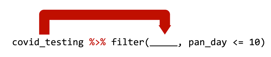
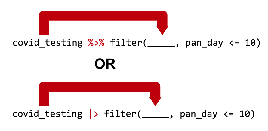
covid_testing %>% filter(pan_day <= 10) is equivalent to filter(covid_testing, pan_day <= 10)
OR, if you in the future use the “new” pipe:
covid_testing |> filter(pan_day <= 10) is equivalent to filter(covid_testing, pan_day <= 10)
Both pipe operators pass the object on its left as the first argument to the function on its right .
In this workshop, we’ll use the “original” pipe (that’s the one that has percent greater than percent) in code examples and quiz questions, because we think this is the one you’ll see the most in code that your coworkers share with you or you find in online examples. We’re also running on the latest stable version of R that ships with our server software, which is 3.6. This will gradually change, and when we get 4.1.0 as the default R version, we’ll likely change these materials to reflect that.
That means, and I’m going to read the top line of code in blue, that the statement “covid_testing, pipe, filter such that pan_day is less than or equal to ten” is equivalent to “filter the covid_testing data frame such that pan day is less than or equal to ten”. Those two lines of code are equivalent.
In both cases we’re taking the covid_testing data frame, passing it as the first argument to the filter() function, and adding a condition that we’re filtering by. In our case that condition is pan_day less than or equal to 10.
We could say the same thing of the second line of blue code on your screen which uses the newer pipe.
This is the last time you’ll see that new pipe today… from here out we’re going to use the old favorite percent greater than percent.
Start with the covid_testing data frame. THEN
Select so that we get only certain columns. THEN
Filter so that we get only certain rows.
Here’s why the pipe (%>% or |>) is so useful.
“Tidy” functions like select(), filter(), and others we’ll see later always have as first argument a data frame, and they always return a data frame as well. Data frame in, data frame out.
This makes it possible to create a pipeline in which a data frame object is handed from one dplyr function to the next. The data frame result of step 1 becomes the data frame starting point for step 2, then the result of step 2 becomes the starting point for step 3, and so on.
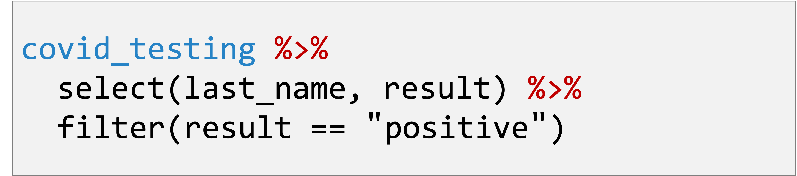
For example, here we start with covid_testing, then select the last_name and result columns, then filter to get rows where result is equal to “positive”.
You might wonder why we’ve put each step in its own line. Is this a requirement? No, it’s not. Many R users like to use whitespace (new lines, tabs, spaces, indents) to make their code more human readable.
By connecting logical steps, you can get a pipeline of data analysis steps which are concise and also fairly human readable. You can think of the pipe symbol as the word “then…”, describing the steps in order.
This approach to coding is powerful because it makes it much easier for someone who doesn’t know R well to read and understand your code as a series of instructions.
Your Turn #4
Rewrite the following statement with a pipe:
select(mydata, first_name, last_name)
Type the answer in the chat!
OK, I want to see if you grasp this concept, as it’s pretty important, moving forward. How would you rewrite the statement on your screen, select mydata comma first name comma last name, and use the pipe syntax instead? Share what you think the answer is.
…
Yep, that’s exactly right! You’d write mydata, the pipe symbol, and then select first name comma last name. Any questions on that?
Create or Update Columns
Let’s say you want to add a new column to your data frame, or update a column by changing it in some way (say, convert kilograms to pounds). dplyr has a function for that, too!
mutate()
Create new or updated, optionally calculated columns.
mutate() is an extremely useful dplyr function, and you can use it to make new variables / columns. That’s what we’ll use it for here. You can also use mutate() to change existing columns (say, turn an entire column lowercase or round or scale a numeric value).
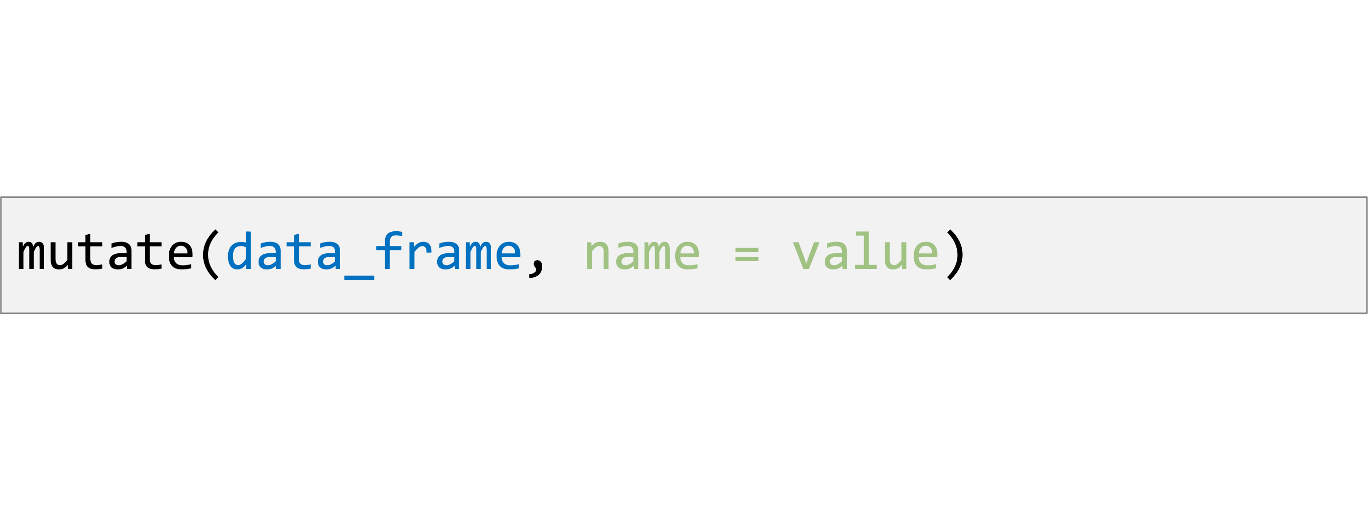
Like all dplyr functions, mutate() takes a data frame as its first argument. After that, you tell it what to name the new column and what should be in it. This is done using name-value expressions .
In name-value expression , you have:
a name
an equals sign (=), and
a value
mutate()
Create new or updated, optionally calculated columns.
mutate()
Create new or updated, optionally calculated columns.
Then you have a single equals sign - because you’re assigning a value (=), you’re not asking whether two things are equal (==).
mutate()
Create new or updated, optionally calculated columns.
Then you have value . This can be a constant, e.g. 100, or a calculation that involves data from already existing columns.
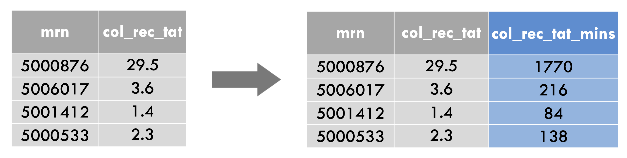
mutate()
mutate(covid_testing,
     col_rec_tat_mins = col_rec_tat * 60)
For example, let’s take a look at one of the columns of covid_testing that we haven’t looked at yet in this workshop: col_rec_tat.
This column contains the specimen collection (“col”) to received-in-lab (“rec”) turn around time (“tat”), in hours. Let’s create a new column, that contains the same data, but in minutes instead of hours.
To do so, you write mutate(covid_testing, followed by a name-value expression. The left part is the new column name, which we could choose to be col_rec_tat_mins. Then we have a single equals sign. Then the calculation, which is col_rec_tat times 60.
mutate()
mutate(covid_testing,
     ct_value = round(ct_value))
If, on the other hand, you wanted to change an existing column using mutate(), you could do it like this. This command takes the column ct_value, which currently holds decimal values, rounds it to the nearest whole number, and then uses that as the new set of values for ct_value.
Your Turn #5
Open 03 – Transform.qmd and work through the exercises.
Click “yes”
Now let’s do some hands-on work. Please go to your “exercises” folder and open the 03 transform file. You’ll have five minutes to go through the instructions in that file!
…
Everyone ready? I’m going to go through the solutions very quickly. In this first exercise, I’ll start with covid_testing, then add a pipe, and then use my filter, making sure I use the double equal. So clinic_name == “picu”. Finally, I’ll add another pipe and then keep only the columns I care about, using select(rec_ver_tat, pan_day).
Then I’ll use mutate without a pipe and make a new column composed of the sum of two existing columns. I’ll do it like this: mutate covid_testing comma total_tat equals col_rec_tat plus rec_ver_tat.
And finally, I’ll take the data frame name out of that mutate and use it as the start of a pipeline. So I have covid_testing, then, mutate, total_tat equals col_rec_tat plus rec_ver_tat.
Recap
select() subsets columns by name
filter() subsets rows by a logical condition
mutate() creates new calculated columns or changes existing columns
Use the pipe operator %>% to combine dplyr functions into a pipeline
To recap, dplyr is a package you can load in R that provides a grammar for transforming data frames. Some of the key dplyr functions are:
select(), which subsets columns by name filter(), which subsets rows by a logical condition , and mutate(), which creates new calculated columns or changes existing columns
Additionally, dplyr and other tidyverse packages make use of the pipe operator, which can be used to string together dplyr functions into a pipeline that performs several transformations.
Cheatsheet (more dplyr functions!)
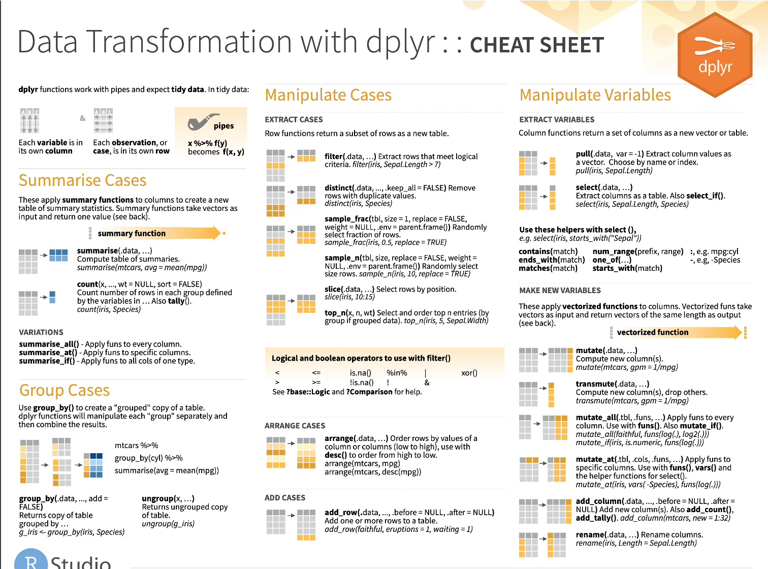
RStudio creates and distributes a number of cheatsheets for various purposes. You can find them by clicking in the Help menu in RStudio – try that now! Here’s an image of the dplyr cheatsheet. As you can see, there are lots of other funtions that dplyr offers.
Other dplyr functions include arrange(), distinct(), group_by() (which is especially helpful when combined with summarize()), and many more!
Beyond dplyr, there are a number of other tidyverse
tidyr provides functions that allow you to convert messy data frames into tidy oneslubridate provides functions to manipulate times and datesstringr provides tools for manipulating text stringspurrr offers advanced functionality to automate complex data transformationsdbplyr allows you to interact with a table inside a database as if it were a data frame


 when you are finished.